
14.3. Silicon with Python#
At a glance
- Goal:
Run the phonon and thermal-conductivity calculations of the Si tutorial from a Python script, and analyze the results with NumPy and Matplotlib.
- You will learn:
how to run anphon from Python dictionaries with
anphon.runhow to read the output files through the returned
Resulthow to get frequencies and eigenvectors at arbitrary \(q\) points with
anphon.Phononhow to read
PREFIX.kappa.h5into a dictionary withResult.h5
- Prerequisites:
The Si tutorial and the
alamode-pythonPython package (see Installation), plus Matplotlib.- Example files:
example/Si/python- Run time:
The whole script takes a few seconds.
The Python package anphon runs the same calculations as the command-line program,
inside the Python process (see anphon (phonon properties) for the full reference).
In this tutorial, we redo the phonon dispersion, phonon DOS, and thermal conductivity of Si from
the Si tutorial with the force constants in example/Si/reference.
The complete script is si_python.py:
It finds the force constants relative to its own location, so it can be run from any directory. The outputs are written to the subdirectories bands, dos, and kappa of the current directory:
$ mkdir si_python && cd si_python
$ python /path/to/alamode/example/Si/python/si_python.py
anphon prints its usual log for each run.
1. Phonon dispersion and DOS#
After the imports, the script locates example/Si/reference:
REF = Path(__file__).resolve().parent.parent / "reference" # example/Si/reference
anphon.run takes one dictionary per input field (general, cell, kpoint, …).
It writes the input file si222.in in workdir and runs it, exactly as anphon si222.in would.
The two runs below are the band structure (KPMODE = 1) and the DOS on a \(20\times 20\times 20\) mesh (KPMODE = 2)
of step 4 of the Si tutorial (DELTA_E = 2 gives a finer energy grid for the DOS than the default 10 cm-1):
# --- Step 1: phonon dispersion and DOS --------------------------------------
fc2 = str(REF / "si222.h5")  # absolute path: anphon runs inside workdir

bands = anphon.run(
    general=dict(PREFIX="si222", MODE="phonons", FCSFILE=fc2),
    kpoint=dict(
        KPMODE=1,
        path=[
            ("G", [0, 0, 0], "X", [0.5, 0.5, 0], 51),
            ("X", [0.5, 0.5, 1], "G", [0, 0, 0], 51),
            ("G", [0, 0, 0], "L", [0.5, 0.5, 0.5], 51),
        ],
    ),
    workdir="bands",
)
dos = anphon.run(
    general=dict(PREFIX="si222", MODE="phonons", FCSFILE=fc2, DELTA_E=2),
    kpoint=dict(KPMODE=2, mesh=[20, 20, 20]),
    workdir="dos",
)
print(bands.files(), dos.files())
Because anphon runs inside workdir, a relative FCSFILE would be looked up there;
the script therefore passes an absolute path.
anphon.format_input(general=..., kpoint=...) returns the input text without running anything,
which is handy to check what will be written.
The returned Result knows the output directory and PREFIX:
bands.files() lists the files si222.* (here ['si222.bands', 'si222.in']; the input file written by run is included)
and bands.path(".bands") gives the path of si222.bands.
The text outputs are read with numpy.loadtxt and plotted with Matplotlib:
# .bands: column 0 is the path coordinate, then 6 branches (cm^-1)
b = np.loadtxt(bands.path(".bands"))
d = np.loadtxt(dos.path(".dos"))  # column 0: frequency (cm^-1), column 1: total DOS
with open(bands.path(".bands")) as f:  # first two lines: labels and their positions
    labels = f.readline().split()[1:]
    ticks = [float(x) for x in f.readline().split()[1:]]

fig, (ax1, ax2) = plt.subplots(
    1,
    2,
    sharey=True,
    figsize=(6, 3.5),
    gridspec_kw=dict(width_ratios=[3, 1], wspace=0.05),
)
ax1.plot(b[:, 0], b[:, 1:], color="C0")
ax1.set_xticks(ticks, [r"$\Gamma$" if s == "G" else s for s in labels])
ax1.set_xlim(ticks[0], ticks[-1])
for t in ticks[1:-1]:
    ax1.axvline(t, color="gray", lw=0.5)
ax1.set_ylabel("Frequency (cm$^{-1}$)")
ax1.set_ylim(0, None)
ax2.plot(d[:, 1], d[:, 0], color="C0")
ax2.set_xlabel("DOS")
ax2.set_xticks([])
ax2.set_xlim(0, None)
fig.savefig("si_phonons.png", dpi=120, bbox_inches="tight")
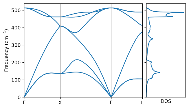
Phonon dispersion and DOS of Si plotted by si_python.py.#
2. Frequencies and eigenvectors at arbitrary q#
anphon.Phonon returns harmonic frequencies and eigenvectors as NumPy arrays for any list of \(q\) points:
# --- Step 2: frequencies and eigenvectors at arbitrary q --------------------
ph = anphon.Phonon(fc2)
q = [[0, 0, 0], [0.5, 0.5, 0], [0.5, 0.5, 0.5]]  # Gamma, X, L (fractional)
w, evec = ph.frequencies(q, eigenvectors=True)
print(w.shape, evec.shape)  # (3, 6) (3, 6, 6)
print(np.round(w, 1))  # cm^-1

# evec[iq, imode, 3 * iatom + ixyz]: the highest mode at Gamma (optical)
# moves the two atoms in opposite directions.
print(np.round(evec[0, 5].reshape(2, 3), 3))
The \(q\) points are given in fractional coordinates of the reciprocal primitive lattice.
The frequencies come in cm-1 with shape (nq, nmodes), where nmodes is three times the number of atoms
in the primitive cell (6 for Si), and the eigenvectors with shape (nq, nmodes, nmodes),
laid out as evec[iq, imode, 3 * iatom + ixyz]. The script prints:
(3, 6) (3, 6, 6)
[[  0.    0.    0.  512.9 512.9 512.9]
 [136.7 136.7 408.8 408.8 461.3 461.3]
 [105.2 105.2 372.5 413.  489.4 489.4]]
[[ 0.631+0.j  0.32 +0.j  0.   +0.j]
 [-0.631+0.j -0.32 +0.j  0.   +0.j]]
The rows are \(\Gamma\), X, and L, and agree with the dispersion above. The last array is the highest mode at \(\Gamma\): the two Si atoms move in opposite directions (optical mode). Since this mode is threefold degenerate, the direction of the displacement within the degenerate subspace is arbitrary.
The force-constant file (HDF5 or XML) carries the species, so kd is optional
(the masses then come from the element table unless MASS is given in general).
The HDF5 file written by alm also carries the primitive cell defined by PRIMCELL in the alm input,
so cell can be omitted as well (pass cell=dict(a=..., lattice=...) for a file fitted without PRIMCELL).
An XML force-constant file does not contain the primitive cell, so cell is always needed for it.
Phonon is quiet by default; pass general=dict(VERBOSITY=1) to see the anphon log.
Ask for all \(q\) points in one call, because each call runs anphon once.
3. Thermal conductivity#
The thermal conductivity in the RTA (step 6 of the Si tutorial) needs the cubic force constants.
The script reads si222_cubic.h5 and runs MODE = kappa in kappa/
on an \(8\times 8\times 8\) mesh, which takes about a second:
# --- Step 3: thermal conductivity on a coarse mesh --------------------------
kdir = Path("kappa")
kdir.mkdir(exist_ok=True)
(kdir / "si222.kappa.h5").unlink(missing_ok=True)  # else anphon restarts from it

res = anphon.run(
    general=dict(
        PREFIX="si222",
        MODE="kappa",
        FCSFILE=str(REF / "si222_cubic.h5"),
        TMIN=100,
        TMAX=1000,
        DT=50,
    ),
    kpoint=dict(KPMODE=2, mesh=[8, 8, 8]),
    workdir=kdir,
)
k = res.h5("kappa")  # the raw contents of si222.kappa.h5
T = k["metadata"]["temperatures"]  # K
kap = k["kappa"]["kappa_peierls"]  # W/mK, shape (nT, 3, 3)
for Ti, ki in zip(T, kap):
    if Ti % 100 == 0:
        print(f"{Ti:6.0f} K {ki[0, 0]:8.1f} W/mK")

fig, ax = plt.subplots(figsize=(4, 3))
ax.plot(T, kap[:, 0, 0], "o-")
ax.set_xlabel("Temperature (K)")
ax.set_ylabel(r"$\kappa$ (W/mK)")
fig.savefig("si_kappa.png", dpi=120, bbox_inches="tight")
res.h5("kappa") reads si222.kappa.h5 into nested dictionaries of NumPy arrays.
The keys are the raw layout of the file described in Thermal conductivity (PREFIX.kappa.h5);
this reader is provisional and may change in a 2.x release (see API stability).
The script prints
 100 K    434.7 W/mK
 200 K    148.2 W/mK
 300 K     90.5 W/mK
 ...
1000 K     26.3 W/mK
The value at 300 K is lower than the result on the \(10\times 10\times 10\) mesh of the Si tutorial (about 104 W/mK).
Change mesh to check the convergence.
The script removes an old si222.kappa.h5 before the run, because anphon would otherwise restart from it
and stop when the mesh differs.
For larger meshes, run the script under MPI as the command-line program:
$ mpirun -np 4 python si_kappa.py
Every anphon.run call is then collective: all ranks must call it with the same arguments.
anphon.Phonon is serial only, so put the kappa run into a script of its own (here si_kappa.py) before using more than one process.
See MPI for details.